Introducing SPARC-fast

Today we are introducing SPARC-fast, our production causal discovery engine. SPARC-fast is a ground-up rebuild of how causal structure is recovered from data, designed for the data organizations actually have: mixed-type, wide, noisy, and large. At scale it is faster than the established methods by three to four orders of magnitude, it is more accurate on the data that defines real-world workloads, and it produces models you can explain.

To measure it, we ran SPARC-fast on the broadest benchmark we have assembled: 69 ground-truth datasets, from 2 to 441 variables, against the established methods of the last three decades and against the winning entries from one of the most recent open causal discovery competitions. Here are the results.

The results#

The 69 datasets are drawn from the bnlearn Bayesian-network repository, the DREAM4 gene-regulatory networks, Microsoft's csuite synthetic benchmarks, the Sachs protein-signalling data and the UCI repository. They span 22 discrete, 37 continuous and 10 mixed-type problems. The full list is in the appendix. The baselines span the history of the field: PC [1], GES [2], hill climbing with LiNGAM [3, 6] and hill climbing with GOLEM [4], the gradient-based successor to NOTEARS [5], each run from its standard implementation.

Every method received a 72-hour compute budget per dataset and was scored coverage-aware: a failure or timeout counts as an empty prediction rather than a quiet exclusion, so no method can lift its average by abstaining on the hardest problems. Where a method exhausted the budget, the budget itself is counted as its runtime, so abstention buys no speed either.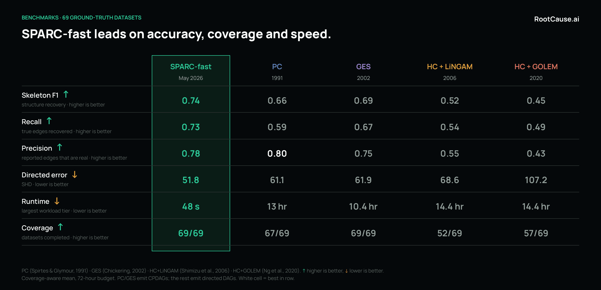Figure 1. Headline comparison across all 69 datasets. Coverage-aware mean, 72-hour budget. Arrows show which direction is better.

The five accuracy terms each answer a different practical question.

Skeleton F1 asks whether a method found the right cause-and-effect links at all, setting aside which way the arrows point; it is the broadest measure of whether the structure is roughly right.

Precision asks how much you can trust what you see: of the links a method reports, what fraction are real? A low score here means chasing relationships that do not exist.

Recall asks the opposite: of the links that are truly there, how many did the method find? A low score means missing the mechanisms you were looking for.

Directed error counts the edits needed to turn the predicted graph into the true one, so it captures the cost of getting directions wrong, not just presence: the difference between knowing two variables are related and knowing which one drives the other.

Coverage asks whether the method finishes at all: how many of the datasets it could complete inside the compute budget. A method that is accurate on the problems it solves but stalls on half of them is not usable in practice.

By these measures, SPARC-fast records the highest skeleton F1 (0.74) and recall (0.73) of any method, the lowest directed error (51.8), and full coverage of all 69 datasets, while running orders of magnitude faster. The rest of this section walks through where those numbers come from.

Accuracy#

SPARC-fast recovers more true causal structure than any other method in the comparison, and it does so while completing every one of the 69 datasets.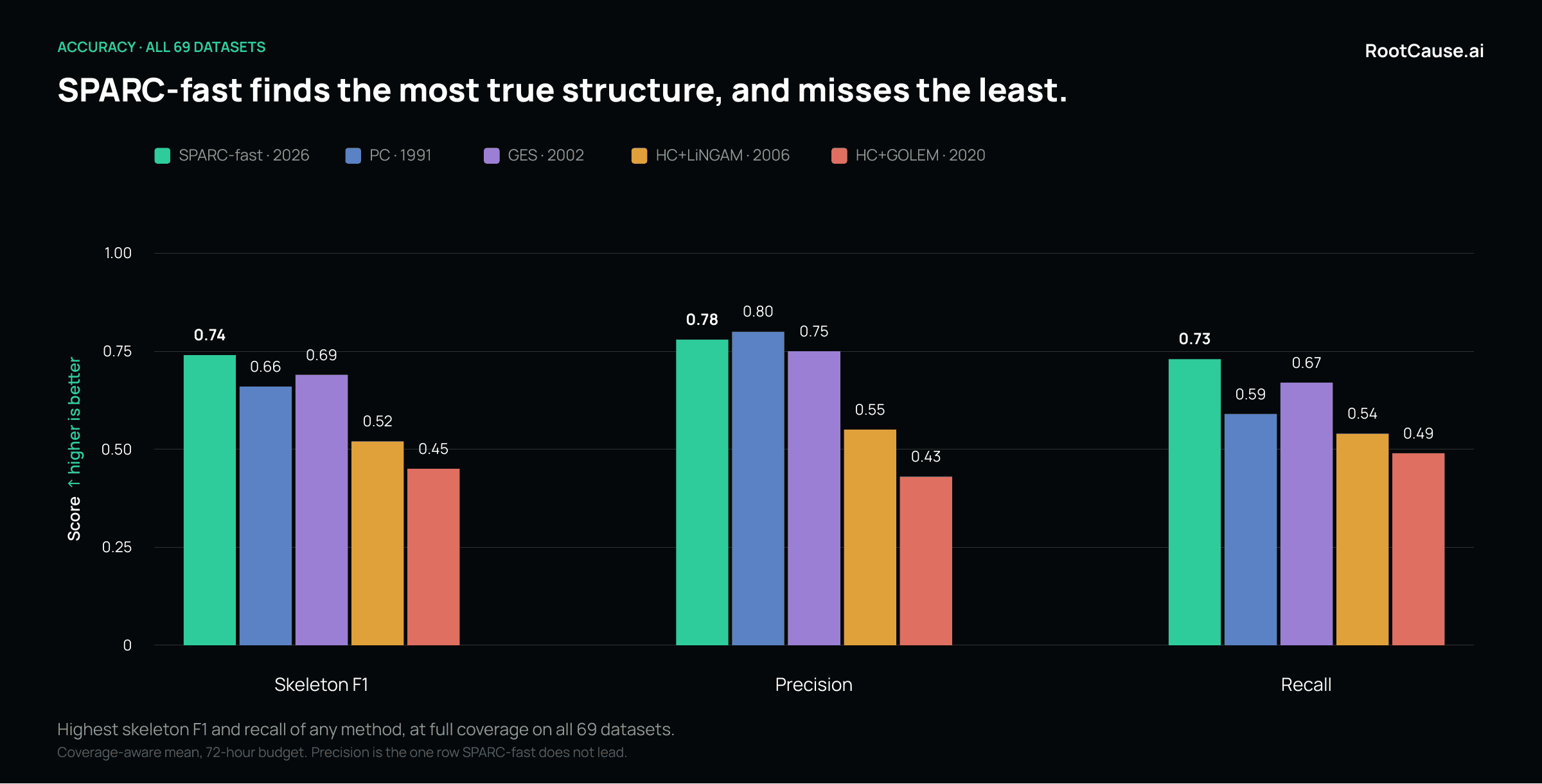Figure 2. Skeleton F1, precision, and recall across the 69 datasets. SPARC-fast posts the highest skeleton F1 and recall of any method.

The one row SPARC-fast does not lead is precision, where PC scores 0.80 to SPARC-fast's 0.78. That is a trade-off: PC asserts a link only when a statistical test clears a significance threshold, so it withholds links it cannot confirm. The same caution drops its recall to 0.59 against SPARC-fast's 0.73: PC reports fewer links and misses more real ones. For a tool meant to answer why and what-if, that trade runs the wrong way, because a reported link can be checked and discarded, but a true relationship the method never surfaces cannot be recovered downstream.

Speed#

SPARC-fast is the fastest unsupervised causal discovery method we know of. At the largest workloads, datasets with hundreds of columns, the other tested methods take 10 to 14 hours per dataset. SPARC-fast takes 48 seconds.

On those largest problems SPARC-fast completed every dataset, while PC, HC+LiNGAM and HC+GOLEM failed or ran out of the 72-hour budget on some of them. Past a few hundred columns, the classical methods stop finishing in a reasonable time.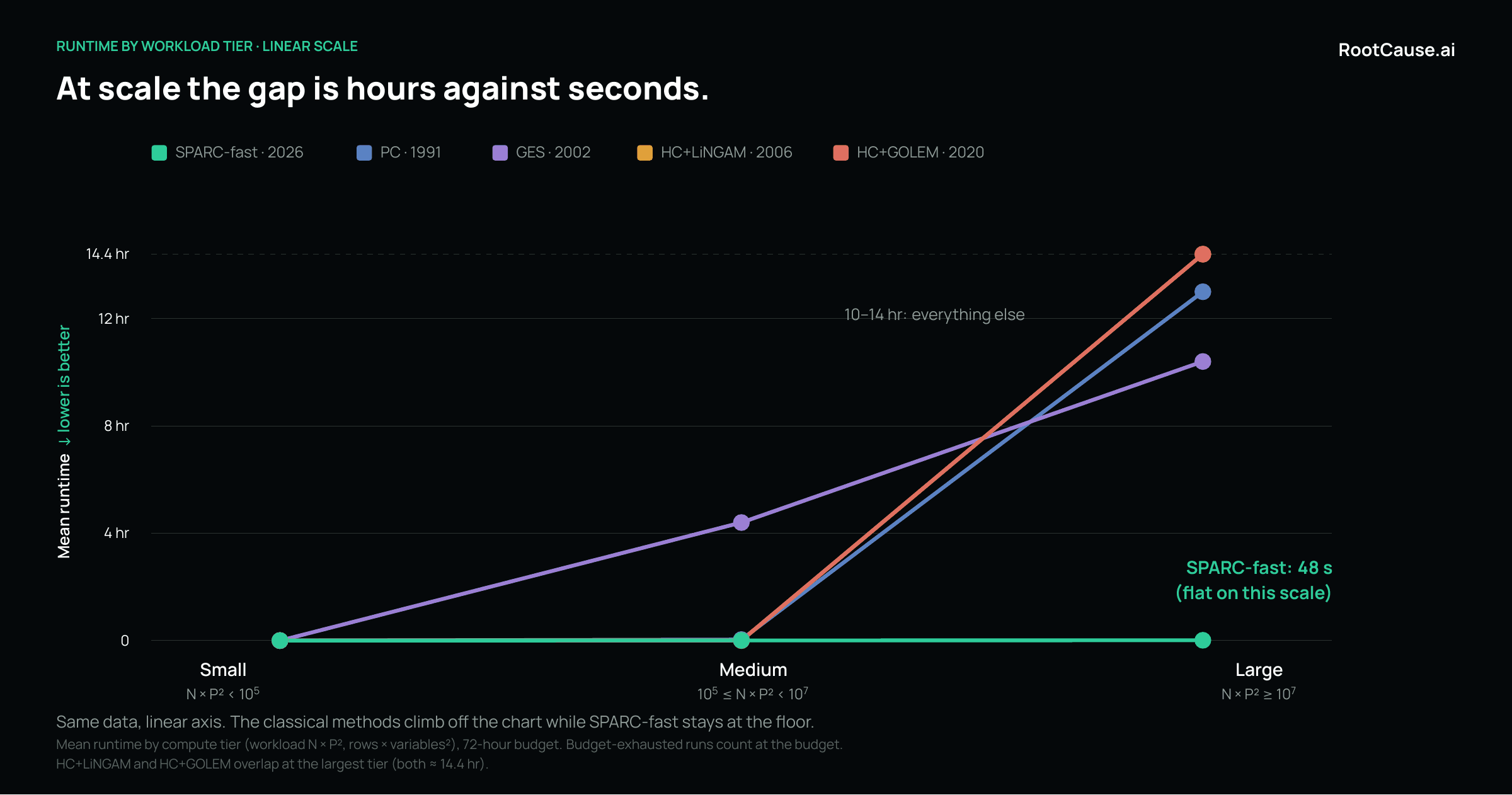Figure 3. Mean runtime by workload tier, linear axis. The classical methods climb off the chart at scale while SPARC-fast stays at the floor.

On a true linear scale, SPARC-fast's runtime is effectively a flat line across the full range of problem sizes. This is the difference between a method run once as an overnight batch job and a method run repeatedly, in the loop of an analysis.

Against the supervised state of the art#

The recent 2024 ADIA Lab Causal Discovery Challenge [12] attracted a number of competitors with models trained on a large corpus of synthetic graphs and then used on real data. We particularly liked the winner of the challenge (who used a scatter and kernel-regression CNN, and the third-place participant (who used a feature and copula-entropy gradient-boosting ensemble). We reproduced their approaches, trained both on the 23,500-graph ADIA corpus, and tested on our benchmark set.

The tested methods scale cubically with the number of variables and were numerically feasible only on 40 small datasets with <=20 variables. Figure 4 reports the comparison with SPARC-fast on this subset. 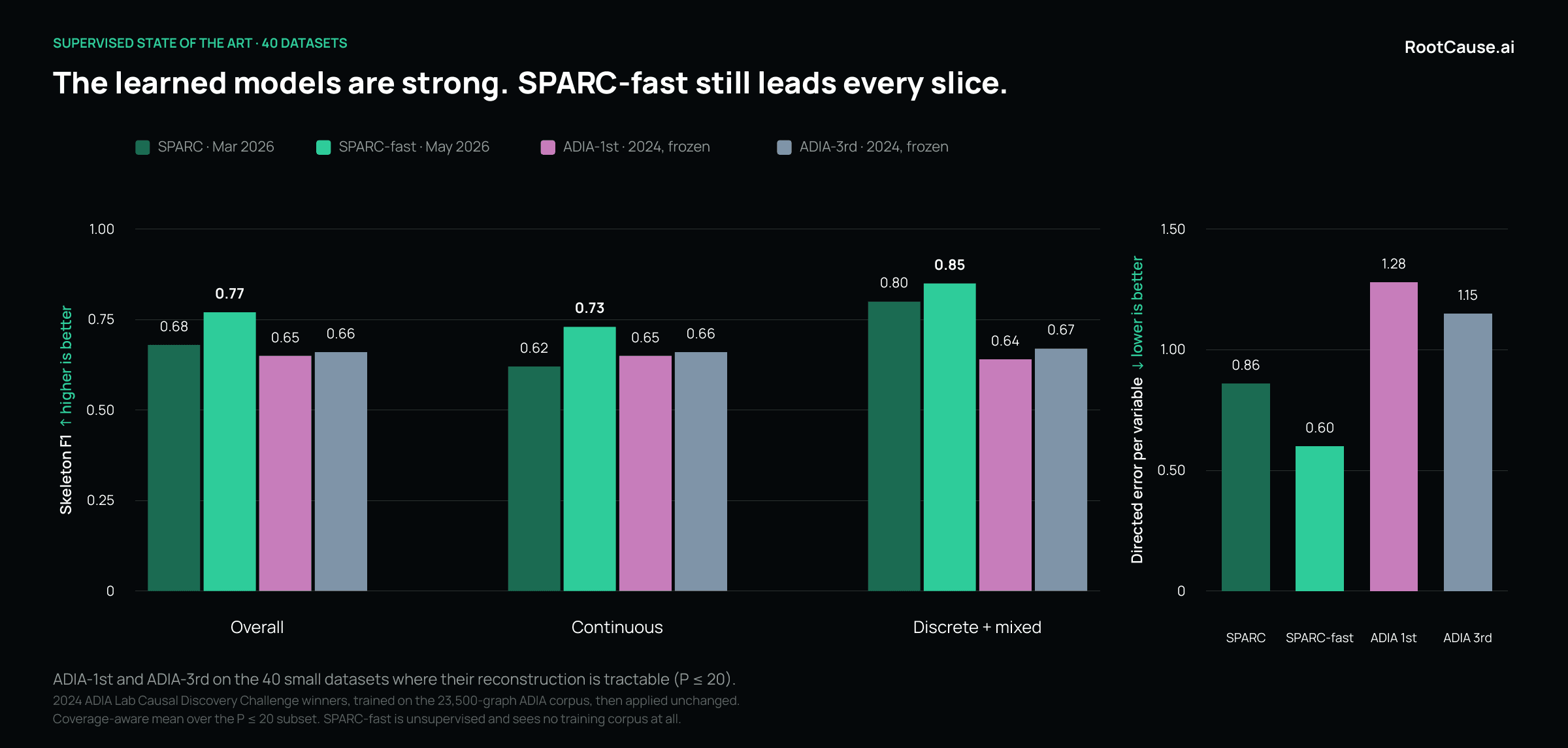Figure 4. SPARC and SPARC-fast against the reproduced ADIA winners, on the 40 small datasets where the reconstruction is tractable. Coverage-aware mean over that subset.

Both learned models recover respectable skeletons, around 0.65 F1. On continuous data resembling the process they were trained on, they are competitive with SPARC, our previous generation. SPARC-fast leads every slice, and the directed error of the learned models is roughly twice as high, because a star-shaped output around a treatment and an outcome does not orient the edges between the remaining variables. SPARC-fast reaches those numbers with no training corpus at all. Why we took the unsupervised route, and what the transfer behaviour of these models tells you about the supervised one, is the subject of a follow-up post, How we got to SPARC-fast.

Does the recovered structure hold up in use?#

Accuracy against a ground-truth graph is one test. A second, more practical test is whether the recovered graph is good enough to work from. A causal graph names, for each variable, the small set of variables that directly drive it, the ones it drives, and the other drivers of those. Statisticians call this set the Markov blanket; in practice it is the shortlist of what matters for that variable.

We tested that shortlist directly. For each dataset we predicted held-out values of every variable three ways: from the Markov blanket in the graph SPARC discovered, from the Markov blanket in the true graph, and with AutoGluon [14], a strong black-box model given every other column in the table. Forecast skill is the held-out R² for numeric targets and the improvement over always guessing the majority class for categorical ones. 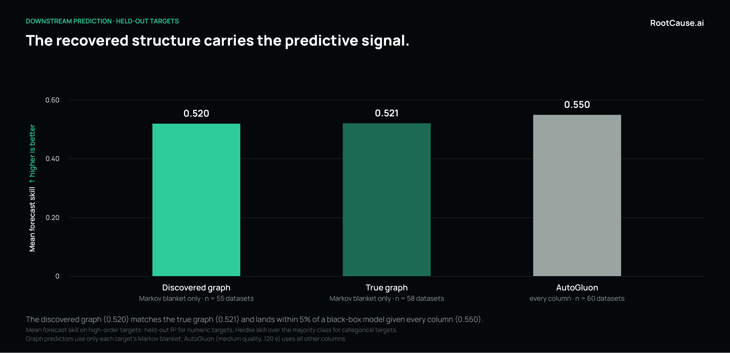Figure 5. Mean forecast skill on the hardest targets. Predicting from the discovered graph's Markov blanket matches the true graph and lands within about 5% of a black-box model that uses every column.

Predicting from the discovered shortlist alone retained about 95% of the skill of the black-box model that saw every column, with a fraction of the inputs and a model whose structure can be explained. More telling is that the discovered graph and the true graph scored the same, an average gap of zero, which indicates that SPARC-fast generally recovers the strongest causal drivers of a variable, the ones that carry its practical predictive signal.

Why causal discovery has stayed in the lab#

Causal discovery recovers cause-and-effect structure directly from data. It answers the two questions correlation cannot: why something happened, and what changes if you intervene. The field has existed since 1991, and its value has never been in question. What has kept it in the research lab is a mismatch between how the methods are built and the data they are asked to run on.

Most causal discovery methods are derived top-down from theoretical assumptions: faithfulness, causal sufficiency, specific noise distributions, no hidden confounders, and often a single variable type. Those assumptions make the mathematics tractable, and they make the methods accurate on the small, tidy, mostly discrete benchmarks the field was developed against. Enterprise data is none of those things. It mixes continuous and categorical columns in one table, runs to hundreds or thousands of variables, carries genuine noise, and routinely hides confounders no one recorded. When the assumptions stop holding, so does the accuracy.

The second barrier is speed. The classical methods build a graph through a sequential search, where each step depends on the result of the last. That structure is hard to parallelize and scales poorly, and on real-world data it pushes runtimes into hours or days for a single problem. A method that runs overnight cannot be a tool an analyst reaches for in the moment. It also cannot be improved quickly, because every research iteration inherits the same wait.

How SPARC-fast is built#

SPARC-fast starts from the data and the outcome rather than from a set of assumptions. It treats mixed-type, noisy, high-dimensional data as the common case, because in practice it is, where several of the established methods have no mechanism for mixed-type data at all.

The name describes the architecture. SPARC is a Screening, Pruning, Agreement and Reconciliation Cascade. Instead of running one expensive procedure across every possible relationship, it moves through stages that grow progressively more expensive and more selective, so the heavy statistics only ever touch the small set of relationships that survive the cheap ones. Four ideas define it.

A cascade that spends compute where it matters. The early stages use inexpensive statistics, with guarantees that protect against discarding real relationships, to screen and prune the large majority of candidate links that are clearly not causal. The expensive tests run only on what survives, and a final agreement and reconciliation stage resolves the result into a coherent directed graph. The classical methods pay the cost of an expensive test across a combinatorial number of relationships, which is the root of their runtime. SPARC inverts the order: cheap and safe first, expensive and selective last.

Functional-form detection that shrinks the search space. Early in the cascade, SPARC identifies the form of the relationships present in the data, which collapses the space of structures it has to consider. This is much of why its cost grows sub-quadratically in the number of variables, where the established methods grow far faster. Sub-quadratic scaling in the variable count is the central breakthrough. It is what moves causal discovery from a problem that explodes with dimensionality into one that stays tractable on the wide tables real organizations have.

An embarrassingly parallel core. Each stage decomposes into independent units of work that run all at once across many distributed cores or a GPU, where the classical sequential search resists parallelization. Combined with the cascade, this is what takes runtime from hours to seconds on the largest problems, growing close to linearly in the number of rows.

Randomized low-rank approximation. Where the expensive statistics do run, SPARC approximates them with randomized low-rank methods and projections that preserve the signal the test depends on while collapsing the work required to compute it.

These choices compound. Because a full evaluation across all 69 datasets runs in minutes rather than weeks, we can run orders of magnitude more experiments, and that iteration velocity is itself how the accuracy was built. We cover that trajectory, and the two research directions we ruled out along the way, in the follow-up post.

What this unlocks#

We built SPARC-fast to make causal discovery accurate out of the box and fast enough to run in seconds. That takes it out of the specialist's overnight queue and makes it the first tool an analyst reaches for when the question is why something happened, or what would change under intervention. It opens a class of problems causal methods have not previously been able to reach: problems that were worked out manually, or handed to correlational tools that quietly give an answer that is wrong and cannot be explained.

For most of its history, causal discovery has been too slow and too narrow for routine use. SPARC-fast was built to change that, and these are the results we are putting forward to be measured against.

References#

1. Spirtes, P. and Glymour, C. (1991). An algorithm for fast recovery of sparse causal graphs. Social Science Computer Review, 9(1), 62–72. https://doi.org/10.1177/089443939100900106
2. Chickering, D. M. (2002). Optimal structure identification with greedy search. Journal of Machine Learning Research, 3, 507–554. https://jmlr.org/papers/v3/chickering02b.html
3. Shimizu, S., Hoyer, P. O., Hyvärinen, A. and Kerminen, A. (2006). A linear non-Gaussian acyclic model for causal discovery. Journal of Machine Learning Research, 7, 2003–2030. https://jmlr.org/papers/v7/shimizu06a.html
4. Ng, I., Ghassami, A. and Zhang, K. (2020). On the role of sparsity and DAG constraints for learning linear DAGs. Advances in Neural Information Processing Systems, 33. https://arxiv.org/abs/2006.10201
5. Zheng, X., Aragam, B., Ravikumar, P. and Xing, E. P. (2018). DAGs with NO TEARS: continuous optimization for structure learning. Advances in Neural Information Processing Systems, 31. https://arxiv.org/abs/1803.01422
6. Heckerman, D., Geiger, D. and Chickering, D. M. (1995). Learning Bayesian networks: the combination of knowledge and statistical data. Machine Learning, 20, 197–243. https://doi.org/10.1007/BF00994016
7. Tsamardinos, I., Brown, L. E. and Aliferis, C. F. (2006). The max-min hill-climbing Bayesian network structure learning algorithm. Machine Learning, 65, 31–78. https://doi.org/10.1007/s10994-006-6889-7
8. Scutari, M. (2010). Learning Bayesian networks with the bnlearn R package. Journal of Statistical Software, 35(3). Bayesian network repository: https://www.bnlearn.com/bnrepository/
9. Marbach, D., Schaffter, T., Mattiussi, C. and Floreano, D. (2009). Generating realistic in silico gene networks for performance assessment of reverse engineering methods. Journal of Computational Biology, 16(2), 229–239. DREAM4 challenge data: https://www.synapse.org/dream4
10. Geffner, T. et al. (2022). Deep end-to-end causal inference. https://arxiv.org/abs/2202.02195. csuite datasets: https://github.com/microsoft/csuite
11. Sachs, K., Perez, O., Pe'er, D., Lauffenburger, D. A. and Nolan, G. P. (2005). Causal protein-signaling networks derived from multiparameter single-cell data. Science, 308(5721), 523–529. https://doi.org/10.1126/science.1105809
12. ADIA Lab Causal Discovery Challenge (2024), hosted by CrunchDAO. https://hub.crunchdao.com/competitions/causality-discovery
13. UCI Machine Learning Repository, Pittsburgh Bridges dataset. https://archive.ics.uci.edu/dataset/18/pittsburgh+bridges
14. Erickson, N. et al. (2020). AutoGluon-Tabular: robust and accurate AutoML for structured data. https://arxiv.org/abs/2003.06505
15. Guyon, I. et al. LUCAS (Lung Cancer Simple Set), Causality Workbench. http://www.causality.inf.ethz.ch/data/LUCAS.html

Appendix: the 69 benchmark datasets#

P is the number of variables, N the number of rows, E the number of ground-truth edges.

dataset	source	type	P	N	E
csuite_cat_chain	csuite [10]	discrete	3	4000	2
csuite_cat_collider	csuite [10]	discrete	3	4000	2
sprinkler	textbook network	discrete	4	1000	4
cancer	bnlearn [8]	discrete	5	10000	4
earthquake	bnlearn [8]	discrete	5	10000	4
survey	bnlearn [8]	discrete	6	10000	6
asia	bnlearn [8]	discrete	8	10000	8
lucas	Causality Workbench [15]	discrete	12	2000	12
child	bnlearn [8]	discrete	20	10000	25
insurance	bnlearn [8]	discrete	27	10000	52
water	bnlearn [8]	discrete	32	10000	66
mildew	bnlearn [8]	discrete	35	10000	46
alarm	bnlearn [8]	discrete	37	10000	46
barley	bnlearn [8]	discrete	48	10000	84
hailfinder	bnlearn [8]	discrete	56	10000	66
hepar2	bnlearn [8]	discrete	70	10000	123
win95pts	bnlearn [8]	discrete	76	10000	112
pathfinder	bnlearn [8]	discrete	109	10000	195
munin1	bnlearn [8]	discrete	186	10000	273
andes	bnlearn [8]	discrete	223	10000	338
diabetes	bnlearn [8]	discrete	413	10000	602
pigs	bnlearn [8]	discrete	441	10000	592
csuite_linexp	csuite [10]	continuous	2	4000	1
csuite_lingauss	csuite [10]	continuous	2	4000	1
csuite_nonlingauss	csuite [10]	continuous	2	4000	1
csuite_nonlin_simpson	csuite [10]	continuous	4	2000	4
csuite_symprod_simpson	csuite [10]	continuous	4	2000	4
csuite_large_backdoor	csuite [10]	continuous	9	2000	9
csuite_weak_arrows	csuite [10]	continuous	9	2000	15
dream4_10_1 … dream4_10_5 (5 networks)	DREAM4 [9]	continuous	10	30	12–16
sachs_1 … sachs_14 (14 experimental conditions)	Sachs [11]	continuous	11	707–927	17
sachs_all	Sachs [11]	continuous	11	11672	17
synth_triples	RootCause synthetic	continuous	13	2000	6
magic_niab	bnlearn [8]	continuous	44	10000	66
ecoli70	bnlearn [8]	continuous	46	10000	70
magic_irri	bnlearn [8]	continuous	64	10000	102
dream4_100_1 … dream4_100_5 (5 networks)	DREAM4 [9]	continuous	100	100	176–249
arth150	bnlearn [8]	continuous	107	10000	150
csuite_cat_to_cts	csuite [10]	mixed	2	4000	1
csuite_cts_to_cat	csuite [10]	mixed	2	4000	1
csuite_mixed_simpson	csuite [10]	mixed	4	4000	4
csuite_large_backdoor_binary_t	csuite [10]	mixed	9	2000	9
csuite_weak_arrows_binary_t	csuite [10]	mixed	9	2000	15
csuite_mixed_confounding	csuite [10]	mixed	12	4000	15
pittsburgh_bridges	UCI [13]	mixed	12	108	4
sangiovese	bnlearn [8]	mixed	15	10000	55
mehra	bnlearn [8]	mixed	24	10000	71
rivers_flood	hydrological network (to confirm)	mixed	42	3010	42